So whenever I have a new blog post, it will be sent to your email (after I edit it).
This is different from my weekly Saturday newsletter.
My blog posts are mostly technical tutorials.
To not miss a post like this, sign up for my newsletter to learn computational
biology and bioinformatics.
What is partial correlation
Partial correlation measures the relationship between two variables while controlling for the effect of one or more other variables.
Suppose you want to know how X and Y are related, independent of how both are influenced by Z. Partial correlation helps answer:
If we remove the influence of Z, is there still a connection between X and Y?
What does it have to do with Bioinformatics?
You are studying the relationship between two genes:
Gene A and Gene B
You observe a high correlation between their expression levels across many samples.
But… both genes might be regulated by Transcription Factor X.
So, is the correlation between Gene A and Gene B direct, or is it just because both are influenced by TF X?
Use partial correlation to test the relationship between Gene A and Gene B, controlling for TF X.
A dummy example in calculating pearson correlation
It is easy to calculate correlation in R with the cor function.
To calculate partial correlation, we will turn to linear regression. What’s the relationship
of linear regression with correlation?
I encourage everyone read this Common statistical tests are linear models.
It shows the linear models underlying common parametric and “non-parametric” tests.
I will walk you through an example in the link above:
# Load packages for data handling and plotting
library(tidyverse)
library(patchwork)
library(broom) # tidy model output
library(kableExtra) # nice table
# Reproducible "random" results
set.seed(123)
# Generate normal data with known parameters
rnorm_fixed<- function(N, mu = 0, sd = 1) scale(rnorm(N)) * sd + mu
y<- c(rnorm(15), exp(rnorm(15)), runif(20, min = -3, max = 0))  # Almost zero mean, not normal
x<- rnorm_fixed(50, mu = 0, sd = 1)  # Used in correlation where this is on x-axis
y2<- x * 2 + rnorm(50)
# Long format data with indicator
value = c(y, y2)
group = rep(c('y1', 'y2'), each = 50)
value
#>   [1] -0.56047565 -0.23017749  1.55870831  0.07050839  0.12928774  1.71506499
#>   [7]  0.46091621 -1.26506123 -0.68685285 -0.44566197  1.22408180  0.35981383
#>  [13]  0.40077145  0.11068272 -0.55584113  5.97099235  1.64518111  0.13992942
#>  [19]  2.01648501  0.62326006  0.34375582  0.80414561  0.35843625  0.48244361
#>  [25]  0.53524041  0.18513068  2.31124663  1.16575986  0.32041542  3.50368377
#>  [31] -1.00465442 -2.71547802 -1.84809109 -2.17684907 -0.55607988 -1.65445098
#>  [37] -0.56980694 -0.56283147 -0.61697304 -1.68050494 -0.73657452 -1.11233661
#>  [43] -0.86945280 -2.99812568 -1.57405028 -2.33964334 -1.86055039 -1.16168699
#>  [49] -1.94460627 -2.66659373 -0.68291806 -0.04276485 -2.70999814  4.07998775
#>  [55]  3.92608432 -3.23176985  1.16150604  0.36461222  1.37554546 -1.33991208
#>  [61] -0.27327874  0.06561465 -0.46989453  2.57602440 -1.58258384  3.20820029
#>  [67] -4.36535571 -0.49221693 -0.23172931  1.27279542  0.14340372 -0.63955336
#>  [73] -2.48836915 -2.45402352 -1.99769497  0.85022079  0.97729907 -0.65016344
#>  [79]  1.07879359  3.41875068 -1.10469580 -6.22321486  1.62403278 -1.96482688
#>  [85]  0.18237357  1.50685612 -0.52711916 -2.77116144 -0.68528078 -0.50858194
#>  [91]  1.32977539  1.18283073 -0.91275131  0.88646473 -2.67243128  1.74339325
#>  [97]  0.85705167  1.58252482  1.05483796  0.98965858
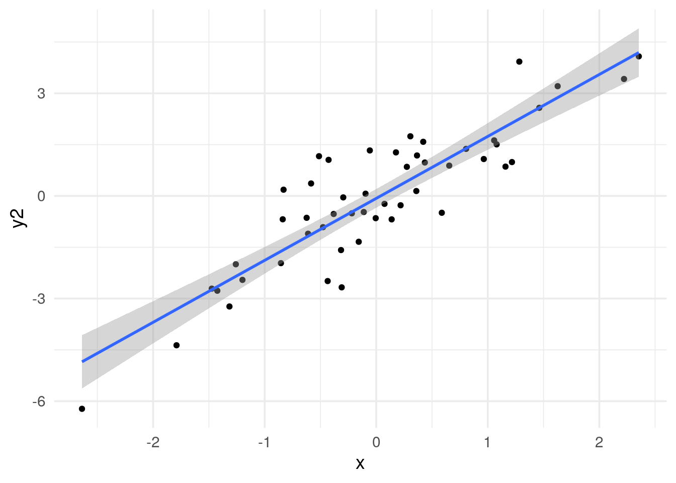
# x and y2 are highly correlated
data.frame(x=x, y=y2) %>%
        ggplot(aes(x=x, y =y2)) +
        geom_point() +
        geom_smooth(method='lm') +
        theme_minimal(base_size = 14)
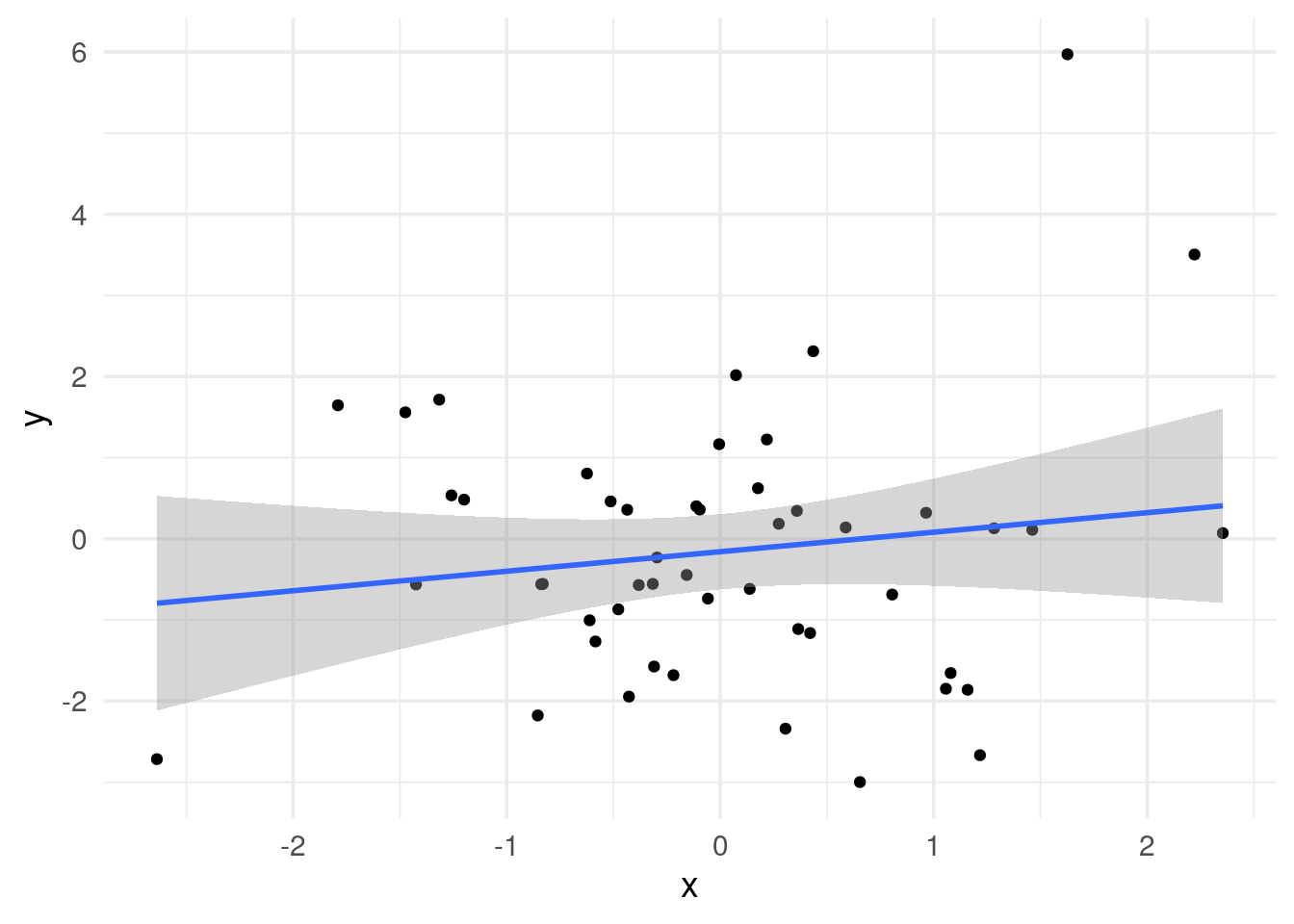
# x and y are not correlated
data.frame(x=x, y=y) %>%
        ggplot(aes(x=x, y =y)) +
        geom_point() +
        geom_smooth(method='lm') +
        theme_minimal(base_size = 14)
Let’s calculate the correlation and p-value
# use cor.test
a<- cor.test(y, x, method = "pearson") # Built-in
a
#>
#> 	Pearson's product-moment correlation
#>
#> data:  y and x
#> t = 1.0303, df = 48, p-value = 0.308
#> alternative hypothesis: true correlation is not equal to 0
#> 95 percent confidence interval:
#>  -0.1368577  0.4087073
#> sample estimates:
#>       cor
#> 0.1470934
tidy(a) %>%
  kable(digits = 3,
        caption = "Correlation Test Results",
        col.names = c("Estimate", "Statistic", "p-value", "Parameter",
                     "Lower CI", "Upper CI", "Method", "Alternative"))
Table 1: Correlation Test Results
| 0.147 |
1.03 |
0.308 |
48 |
-0.137 |
0.409 |
Pearson’s product-moment correlation |
two.sided |
## use linear model
b<- lm(y ~ 1 + x) # Equivalent linear model: y = Beta0*1 + Beta1*x
# Create a nice table
tidy(b) %>%
  kable(digits = 3,
        caption = "Linear Model Results",
        col.names = c("Term", "Estimate", "Std Error", "t-statistic", "p-value"))
Table 1: Linear Model Results
| (Intercept) |
-0.159 |
0.231 |
-0.689 |
0.494 |
| x |
0.241 |
0.233 |
1.030 |
0.308 |
The p-value is the same (p = 0.308), but the coefficient is not (0.147 vs 0.241).
It turns out, we need to standardize x and y to get the same correlation coefficient.
# need to scale to get the same correlation coefficient
c<- lm(scale(y) ~ 1 + scale(x))
tidy(c) %>%
  kable(digits = 3,
        caption = "Linear Model Results",
        col.names = c("Term", "Estimate", "Std Error", "t-statistic", "p-value"))
Table 2: Linear Model Results
| (Intercept) |
0.000 |
0.141 |
0.00 |
1.000 |
| scale(x) |
0.147 |
0.143 |
1.03 |
0.308 |
Now, we get the same 0.147 of the coefficient.
Why need to standardize it to get the right correlation coefficient
Pearson’s Correlation Coefficient
The formula for Pearson’s correlation coefficient (\(r\)) is:
\[
r = \frac{\sum_{i=1}^{n} (x_i - \bar{x})(y_i - \bar{y})}
{\sqrt{\sum_{i=1}^{n} (x_i - \bar{x})^2} \sqrt{\sum_{i=1}^{n} (y_i - \bar{y})^2}}
\]
Regression Slope for Standardized Variables
When \(x\) and \(y\) are standardized to \(z\)-scores:
\[
x_{std} = \frac{x - \bar{x}}{SD(x)}
\]
\[
y_{std} = \frac{y - \bar{y}}{SD(y)}
\]
The regression slope (\(\beta\)) is:
\[
\beta = \frac{\sum_{i=1}^{n} x_{std,i} \, y_{std,i}}{\sum_{i=1}^{n} x_{std,i}^2}
\]
Proof of Equivalence
Since standardized variables have \(SD(x_{std}) = SD(y_{std}) = 1\),
\[
\sum_{i=1}^{n} x_{std,i}^2 = n
\]
So,
\[
\beta = \frac{\sum_{i=1}^{n} x_{std,i} \, y_{std,i}}{n}
\]
Expanding \(x_{std}\) and \(y_{std}\):
\[
\beta = \frac{1}{n} \cdot \frac{\sum_{i=1}^{n} (x_i - \bar{x})(y_i - \bar{y})}{SD(x) \cdot SD(y)}
\]
Therefore,
\[
\beta = r
\]
Now, let’s calculate the pairs of x and y1 which are significantly correlated:
a2<- cor.test(y2, x, method = "pearson") # Built-in
a2
#>
#> 	Pearson's product-moment correlation
#>
#> data:  y2 and x
#> t = 13.164, df = 48, p-value < 2.2e-16
#> alternative hypothesis: true correlation is not equal to 0
#> 95 percent confidence interval:
#>  0.8048173 0.9333683
#> sample estimates:
#>       cor
#> 0.8849249
tidy(a2) %>%
  kable(digits = 3,
        caption = "Correlation Test Results",
        col.names = c("Estimate", "Statistic", "p-value", "Parameter",
                     "Lower CI", "Upper CI", "Method", "Alternative"))
Table 3: Correlation Test Results
| 0.885 |
13.164 |
0 |
48 |
0.805 |
0.933 |
Pearson’s product-moment correlation |
two.sided |
correlation of 0.885 with a p value of 0.
## use linear model
b2<- lm(y2 ~ 1 + x) # Equivalent linear model: y = Beta0*1 + Beta1*x
# Create a nice table
tidy(b2) %>%
  kable(digits = 3,
        caption = "Linear Model Results",
        col.names = c("Term", "Estimate", "Std Error", "t-statistic", "p-value"))
Table 4: Linear Model Results
| (Intercept) |
-0.072 |
0.136 |
-0.526 |
0.601 |
| x |
1.811 |
0.138 |
13.164 |
0.000 |
# need to scale to get the same correlation coefficient
c2<- lm(scale(y2) ~ 1 + scale(x))
tidy(c2) %>%
  kable(digits = 3,
        caption = "Linear Model Results",
        col.names = c("Term", "Estimate", "Std Error", "t-statistic", "p-value"))
Table 5: Linear Model Results
| (Intercept) |
0.000 |
0.067 |
0.000 |
1 |
| scale(x) |
0.885 |
0.067 |
13.164 |
0 |
we get the same coefficient of 0.885 and p-value of 0.
It is very satisfying to see we get the same results using different methods.
A practical example in calculating partial correlation
Go to Depmap
Download the CRISPR screening dependency data CRISPRGeneEffect.csv
The file is > 400MB.
Also download the Model.csv file which contains the metadata information (e.g, cancer type for each cell line)
library(readr)
library(dplyr)
#read in the data
crispr_score<- read_csv("~/blog_data/CRISPRGeneEffect.csv")
crispr_score[1:5, 1:5]
#> # A tibble: 5 × 5
#>   ...1       `A1BG (1)` `A1CF (29974)` `A2M (2)` `A2ML1 (144568)`
#>
We need to clean up the column names. remove the parentheses and the ENTREZE ID (numbers).
NOTE: this type of regular expression is a perfect question for LLM.
crispr_score<- crispr_score %>%
        dplyr::rename(ModelID = `...1`) %>%
        rename_with(~str_trim(str_remove(.x, " \(.*\)$")), -1)
crispr_score[1:5, 1:5]
#> # A tibble: 5 × 5
#>   ModelID       A1BG     A1CF     A2M   A2ML1
#>
meta<- read_csv("~/blog_data/Model.csv")
head(meta)
#> # A tibble: 6 × 47
#>   ModelID    PatientID CellLineName StrippedCellLineName DepmapModelType
#>
table(meta$OncotreeLineage)
#>
#>             Adrenal Gland          Ampulla of Vater             B lymphoblast
#>                         2                         4                         1
#>             Biliary Tract     Bladder/Urinary Tract                      Bone
#>                        46                        39                        90
#>                     Bowel                    Breast                    Cervix
#>                        99                        96                        25
#>                 CNS/Brain                 Embryonal         Esophagus/Stomach
#>                       125                         1                       103
#>                       Eye                Fibroblast                      Hair
#>                        24                        42                         2
#>             Head and Neck                    Kidney                     Liver
#>                        95                        73                        29
#>                      Lung                  Lymphoid                    Muscle
#>                       260                       260                         5
#>                   Myeloid                    Normal                     Other
#>                        88                        13                         2
#>      Ovary/Fallopian Tube                  Pancreas Peripheral Nervous System
#>                        75                        68                        60
#>                    Pleura                  Prostate                      Skin
#>                        36                        15                       149
#>               Soft Tissue                    Testis                   Thyroid
#>                        86                        12                        25
#>                    Uterus              Vulva/Vagina
#>                        44                         5
# subset only the breast cancer cell line
breast_meta<- meta %>%
        select(ModelID, OncotreeLineage) %>%
        mutate(breast = case_when(
                OncotreeLineage == "Breast" ~ "yes",
                TRUE ~ "no"
        ))
crispr_all<- inner_join(meta, crispr_score)
crispr_all<- crispr_all %>%
        mutate(breast = case_when(
                OncotreeLineage == "Breast" ~ "yes",
                TRUE ~ "no"
        ))
ggplot(crispr_all,  aes(x= FOXA1, y= ESR1)) +
        geom_point(aes(color = breast)) +
        geom_smooth(method='lm', formula= y~x) +
        facet_wrap(~breast)
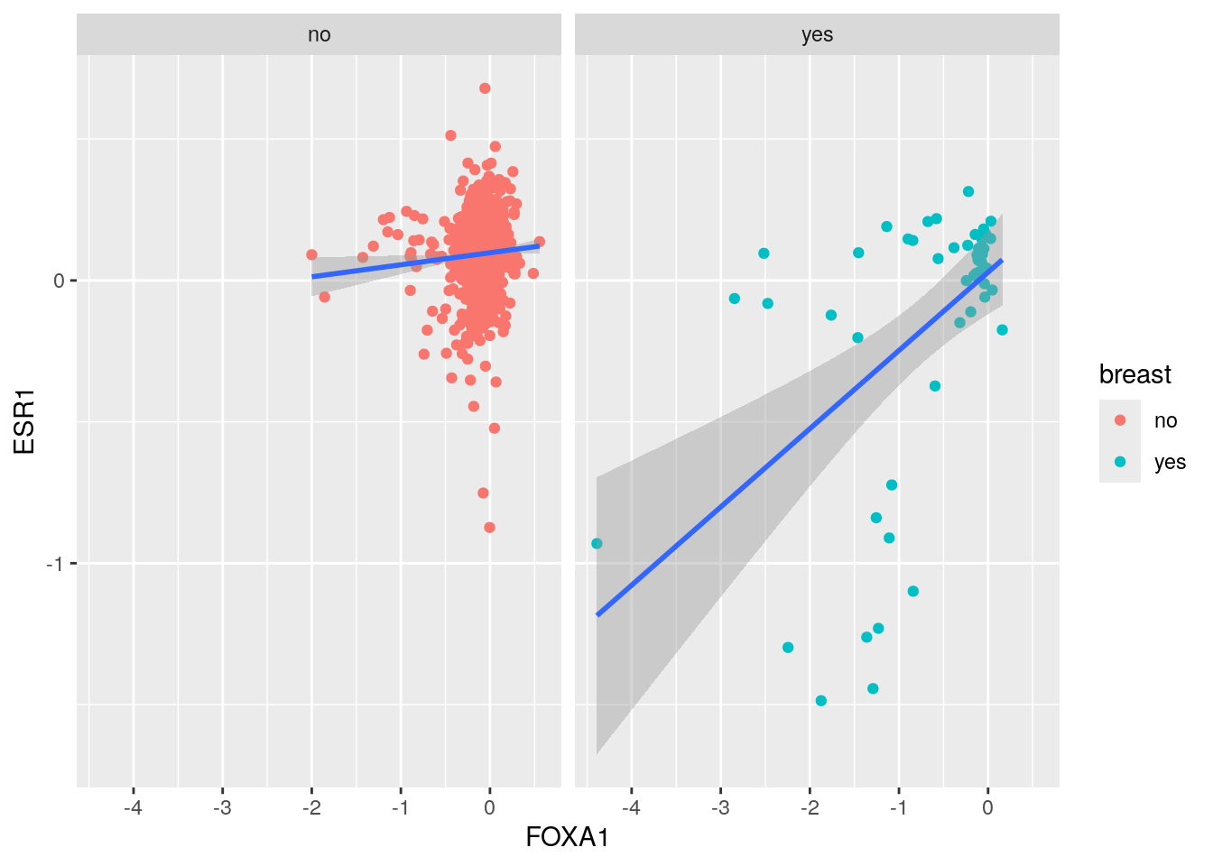 It looks like the FOXA1 and ESR1 CRISPR dependency score are more correlated in Breast cancer.
Let’s calculate the correlation and p-value
cor.test(crispr_all$FOXA1[crispr_all$breast == "yes"], crispr_all$ESR1[crispr_all$breast == "yes"])
#>
#> 	Pearson's product-moment correlation
#>
#> data:  crispr_all$FOXA1[crispr_all$breast == "yes"] and crispr_all$ESR1[crispr_all$breast == "yes"]
#> t = 4.3022, df = 51, p-value = 7.658e-05
#> alternative hypothesis: true correlation is not equal to 0
#> 95 percent confidence interval:
#>  0.2855579 0.6900675
#> sample estimates:
#>       cor
#> 0.5160227
cor.test(crispr_all$FOXA1, crispr_all$ESR1)
#>
#> 	Pearson's product-moment correlation
#>
#> data:  crispr_all$FOXA1 and crispr_all$ESR1
#> t = 14.076, df = 1176, p-value < 2.2e-16
#> alternative hypothesis: true correlation is not equal to 0
#> 95 percent confidence interval:
#>  0.3297560 0.4275629
#> sample estimates:
#>       cor
#> 0.3797201
All cell lines (r = 0.38): This includes the confounding effect of cancer type. Different cancer types have different baseline dependencies for both FOXA1 and ESR1.
Breast cancer only (r = 0.52): This removes the cancer type confounding, showing the “true” relationship within a homogeneous cancer type.
The increase from 0.38 to 0.52 suggests that cancer type was acting as a confounding variable, diluting the true correlation between FOXA1 and ESR1 dependencies.
Let’s use linear model to calculate correlation
# need to scale to get the same correlation coefficient
lm_cor <- lm(scale(crispr_all$ESR1) ~ 1 + scale(crispr_all$FOXA1))
summary(lm_cor)
#>
#> Call:
#> lm(formula = scale(crispr_all$ESR1) ~ 1 + scale(crispr_all$FOXA1))
#>
#> Residuals:
#>     Min      1Q  Median      3Q     Max
#> -7.7928 -0.3632  0.0598  0.4546  3.5335
#>
#> Coefficients:
#>                          Estimate Std. Error t value Pr(>|t|)
#> (Intercept)             4.703e-17  2.697e-02    0.00        1
#> scale(crispr_all$FOXA1) 3.797e-01  2.698e-02   14.08   <2e-16 ***
#> ---
#> Signif. codes:  0 '***' 0.001 '**' 0.01 '*' 0.05 '.' 0.1 ' ' 1
#>
#> Residual standard error: 0.9255 on 1176 degrees of freedom
#> Multiple R-squared:  0.1442,	Adjusted R-squared:  0.1435
#> F-statistic: 198.1 on 1 and 1176 DF,  p-value: < 2.2e-16
# a nice table
tidy(lm_cor) %>%
  kable(digits = 3,
        caption = "Linear Model Results",
        col.names = c("Term", "Estimate", "Std Error", "t-statistic", "p-value"))
Table 6: Linear Model Results
| (Intercept) |
0.00 |
0.027 |
0.000 |
1 |
| scale(crispr_all$FOXA1) |
0.38 |
0.027 |
14.076 |
0 |
The results is the same as cor.test(crispr_all$FOXA1, crispr_all$ESR1)
adding the cancer type as a covariate to calculate partial correlation
lm_cor_partial <- lm(scale(crispr_all$ESR1) ~ scale(crispr_all$FOXA1) + crispr_all$OncotreeLineage)
unique(crispr_all$OncotreeLineage) %>% sort()
#>  [1] "Adrenal Gland"             "Ampulla of Vater"
#>  [3] "Biliary Tract"             "Bladder/Urinary Tract"
#>  [5] "Bone"                      "Bowel"
#>  [7] "Breast"                    "Cervix"
#>  [9] "CNS/Brain"                 "Esophagus/Stomach"
#> [11] "Eye"                       "Fibroblast"
#> [13] "Head and Neck"             "Kidney"
#> [15] "Liver"                     "Lung"
#> [17] "Lymphoid"                  "Myeloid"
#> [19] "Other"                     "Ovary/Fallopian Tube"
#> [21] "Pancreas"                  "Peripheral Nervous System"
#> [23] "Pleura"                    "Prostate"
#> [25] "Skin"                      "Soft Tissue"
#> [27] "Testis"                    "Thyroid"
#> [29] "Uterus"                    "Vulva/Vagina"
We have 30 lineages, and by default the reference group is Adrenal Gland which is the first sorted alphabetically.
summary(lm_cor_partial)
#>
#> Call:
#> lm(formula = scale(crispr_all$ESR1) ~ scale(crispr_all$FOXA1) +
#>     crispr_all$OncotreeLineage)
#>
#> Residuals:
#>     Min      1Q  Median      3Q     Max
#> -7.1693 -0.3711  0.0329  0.4560  3.5215
#>
#> Coefficients:
#>                                                     Estimate Std. Error t value
#> (Intercept)                                           1.2382     0.9029   1.371
#> scale(crispr_all$FOXA1)                               0.3021     0.0299  10.104
#> crispr_all$OncotreeLineageAmpulla of Vater           -0.9696     1.0094  -0.961
#> crispr_all$OncotreeLineageBiliary Tract              -1.2050     0.9157  -1.316
#> crispr_all$OncotreeLineageBladder/Urinary Tract      -1.0857     0.9161  -1.185
#> crispr_all$OncotreeLineageBone                       -1.1071     0.9126  -1.213
#> crispr_all$OncotreeLineageBowel                      -1.0521     0.9100  -1.156
#> crispr_all$OncotreeLineageBreast                     -2.1645     0.9131  -2.371
#> crispr_all$OncotreeLineageCervix                     -0.8041     0.9276  -0.867
#> crispr_all$OncotreeLineageCNS/Brain                  -1.3465     0.9079  -1.483
#> crispr_all$OncotreeLineageEsophagus/Stomach          -1.1176     0.9094  -1.229
#> crispr_all$OncotreeLineageEye                        -1.3322     0.9325  -1.429
#> crispr_all$OncotreeLineageFibroblast                 -0.8213     1.2769  -0.643
#> crispr_all$OncotreeLineageHead and Neck              -1.1233     0.9087  -1.236
#> crispr_all$OncotreeLineageKidney                     -1.4100     0.9161  -1.539
#> crispr_all$OncotreeLineageLiver                      -1.0757     0.9215  -1.167
#> crispr_all$OncotreeLineageLung                       -1.2399     0.9064  -1.368
#> crispr_all$OncotreeLineageLymphoid                   -1.1707     0.9078  -1.290
#> crispr_all$OncotreeLineageMyeloid                    -1.1257     0.9136  -1.232
#> crispr_all$OncotreeLineageOther                      -0.7691     1.2769  -0.602
#> crispr_all$OncotreeLineageOvary/Fallopian Tube       -1.6780     0.9105  -1.843
#> crispr_all$OncotreeLineagePancreas                   -1.1337     0.9124  -1.242
#> crispr_all$OncotreeLineagePeripheral Nervous System  -1.1941     0.9131  -1.308
#> crispr_all$OncotreeLineagePleura                     -1.0867     0.9241  -1.176
#> crispr_all$OncotreeLineageProstate                   -0.8901     0.9481  -0.939
#> crispr_all$OncotreeLineageSkin                       -1.0486     0.9090  -1.154
#> crispr_all$OncotreeLineageSoft Tissue                -1.2275     0.9129  -1.345
#> crispr_all$OncotreeLineageTestis                     -1.9009     0.9891  -1.922
#> crispr_all$OncotreeLineageThyroid                    -1.1388     0.9430  -1.208
#> crispr_all$OncotreeLineageUterus                     -1.2534     0.9161  -1.368
#> crispr_all$OncotreeLineageVulva/Vagina               -1.3165     1.1058  -1.191
#>                                                     Pr(>|t|)
#> (Intercept)                                           0.1705
#> scale(crispr_all$FOXA1)                               <2e-16 ***
#> crispr_all$OncotreeLineageAmpulla of Vater            0.3370
#> crispr_all$OncotreeLineageBiliary Tract               0.1884
#> crispr_all$OncotreeLineageBladder/Urinary Tract       0.2362
#> crispr_all$OncotreeLineageBone                        0.2254
#> crispr_all$OncotreeLineageBowel                       0.2479
#> crispr_all$OncotreeLineageBreast                      0.0179 *
#> crispr_all$OncotreeLineageCervix                      0.3862
#> crispr_all$OncotreeLineageCNS/Brain                   0.1383
#> crispr_all$OncotreeLineageEsophagus/Stomach           0.2193
#> crispr_all$OncotreeLineageEye                         0.1534
#> crispr_all$OncotreeLineageFibroblast                  0.5203
#> crispr_all$OncotreeLineageHead and Neck               0.2167
#> crispr_all$OncotreeLineageKidney                      0.1240
#> crispr_all$OncotreeLineageLiver                       0.2433
#> crispr_all$OncotreeLineageLung                        0.1716
#> crispr_all$OncotreeLineageLymphoid                    0.1974
#> crispr_all$OncotreeLineageMyeloid                     0.2182
#> crispr_all$OncotreeLineageOther                       0.5471
#> crispr_all$OncotreeLineageOvary/Fallopian Tube        0.0656 .
#> crispr_all$OncotreeLineagePancreas                    0.2143
#> crispr_all$OncotreeLineagePeripheral Nervous System   0.1912
#> crispr_all$OncotreeLineagePleura                      0.2399
#> crispr_all$OncotreeLineageProstate                    0.3481
#> crispr_all$OncotreeLineageSkin                        0.2489
#> crispr_all$OncotreeLineageSoft Tissue                 0.1790
#> crispr_all$OncotreeLineageTestis                      0.0549 .
#> crispr_all$OncotreeLineageThyroid                     0.2274
#> crispr_all$OncotreeLineageUterus                      0.1715
#> crispr_all$OncotreeLineageVulva/Vagina                0.2341
#> ---
#> Signif. codes:  0 '***' 0.001 '**' 0.01 '*' 0.05 '.' 0.1 ' ' 1
#>
#> Residual standard error: 0.9029 on 1147 degrees of freedom
#> Multiple R-squared:  0.2056,	Adjusted R-squared:  0.1848
#> F-statistic: 9.896 on 30 and 1147 DF,  p-value: < 2.2e-16
Interpreting the linear model coefficients
- FOXA1 coefficient (scale(crispr_all$FOXA1) = 0.3021)
Meaning: For every 1 standard deviation increase in FOXA1 dependency score, ESR1 dependency score increases by 0.3021 standard deviations, controlling for cancer type
P-value < 2e-16: Highly significant relationship
This 0.3021 is your partial correlation coefficient between FOXA1 and ESR1, controlling for cancer type
- Cancer type coefficients (e.g., Breast = -2.1645)
Meaning: Each coefficient represents the difference in ESR1 dependency (in standard deviations) between that cancer type and the reference cancer type (Adrenal Gland).
Breast coefficient (-2.1645, p = 0.0179): Breast cancer cell lines have significantly lower ESR1 dependency scores compared to the reference cancer type (Adrenal Gland), on average.
Most other cancer types: Non-significant differences from the reference type.
Biological interpretation:
FOXA1 and ESR1 have a moderate positive partial correlation (0.30) across cancer types.
This suggests these genes may be part of related pathways or have synthetic lethal relationships.
Breast cancer shows even stronger co-dependency (0.53), which makes biological sense given the importance of estrogen signaling in breast cancer.
The significant negative coefficient for breast cancer (-2.16) indicates breast cancers generally have lower ESR1 dependency scores overall.
What we found suggest
FOXA1-ESR1 have genuine co-dependency (partial r = 0.30).
Breast cancer amplifies this relationship (r = 0.53 within breast).
Cancer type was indeed confounding the raw correlation (0.37).
The relationship is biologically meaningful across cancer types, but particularly strong in breast cancer.
Other usages of partial correlation
Partial Correlation Improves Network Accuracy
- Eliminating Spurious Correlations
Problem: Standard Pearson/Spearman correlations detect both direct interactions and indirect relationships mediated by shared regulators or technical confounders (e.g., batch effects).
Solution: Partial correlation removes the linear effects of all other variables, revealing direct dependencies between gene pairs.
- Biological Validation
Studies show partial correlation networks:
Reduce false positives by 30-50% compared to correlation networks in cancer genomics
Align better with experimentally validated interactions (e.g., ChIP-seq/TF binding data).
Further readings:
Tommy aka. crazyhottommy